Detection of Breast Cancer In Biopsy Specimens Using Machine Learning

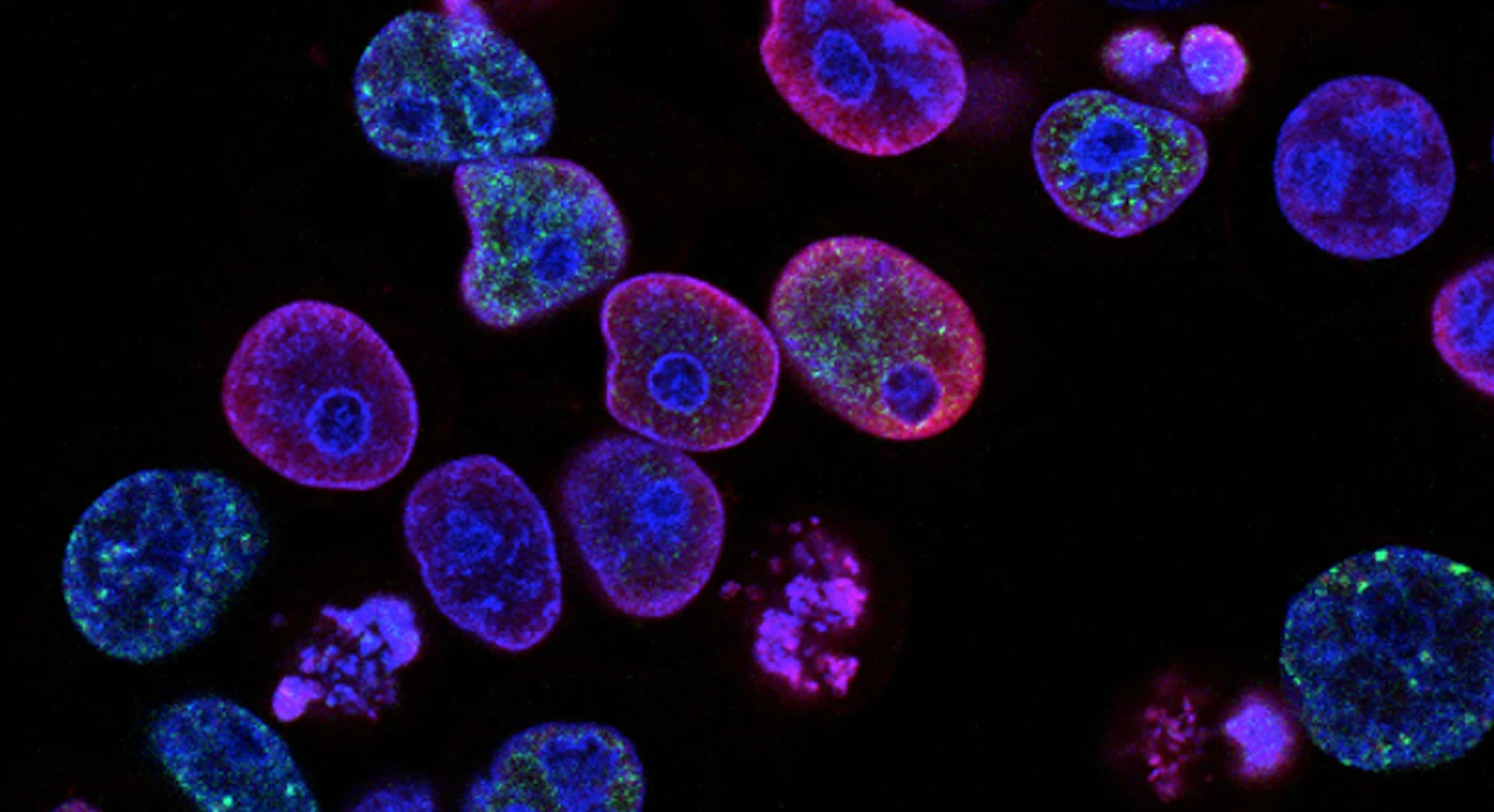
Breast cancer continues to be a significant culprit of morbidity and mortality, even today with our current medical advances. The data that this dataset consists of was actually published in a medical journal article and data was collected at the University of Wisconsin (Wolberg, M.D. et al.¸1995). While this source is somewhat dated, my main goal with this project is to demonstrate that machine learning algorithms could be used to assist in cancer detection as adjunct to physician expertise.

Problem Background:

It is no secret that our healthcare is cumbersome, overpriced, and our outcomes are unsatisfactory when compared to other peer countries. In a data-driven world, with the vast amounts of personal health information and data available in electronic health records, the sky is the limit. Could machine learning algorithms be used to improve diagnosis, save lives, and prevent suffering?

Breast cancer is the second most common cause of death due to cancer in women. Using mammograms, women are screened for breast cancer. Suspicious areas identified radiologically are then biopsied using a wide variety of techniques. One method is using a fine needle aspirate in which cells from the area in question are extracted and examined under the microscope. Even with expert analysis, accurate diagnosis can be challenging.

Therefore, the question remains, can machine learning help us predict malignant tumors as an adjunct to physician expertise?

Dataset Description:

The data is from the University of California - Irvine Machine Learning Repository and can be found here:

https://archive.ics.uci.edu/ml/datasets/Breast+Cancer+Wisconsin+%28Diagnostic%29

This data was collected at the University of Wisconsin in 1995. The file is in a csv format in which microscopic images of Fine Needle Aspirates (a type of biopsy) of suspicious breast tissue was digitized. There are a total of 32 variables with 570 subjects. They were examining suspicious masses in those without evidence of metastasis (distant spread of cancer to other parts of the body).

After data cleaning, exploration, and analysis, the data will be fit and predictive ability evaluated using Logistic Regression, K Nearest Neighbors, and Random Forest machine learning algorithms.

Data Cleaning, Exploration, and Analysis

The dataframe is included below:

	id	diagnosis	radius_mean	texture_mean	perimeter_mean	area_mean	smoothness_mean	compactness_mean	concavity_mean	concave points_mean	...	radius_worst	texture_worst	perimeter_worst	area_worst	smoothness_worst	compactness_worst	concavity_worst	concave points_worst	symmetry_worst	fractal_dimension_worst
0	842302	M	17.99	10.38	122.80	1001.0	0.11840	0.27760	0.30010	0.14710	...	25.380	17.33	184.60	2019.0	0.16220	0.66560	0.7119	0.2654	0.4601	0.11890
1	842517	M	20.57	17.77	132.90	1326.0	0.08474	0.07864	0.08690	0.07017	...	24.990	23.41	158.80	1956.0	0.12380	0.18660	0.2416	0.1860	0.2750	0.08902
2	84300903	M	19.69	21.25	130.00	1203.0	0.10960	0.15990	0.19740	0.12790	...	23.570	25.53	152.50	1709.0	0.14440	0.42450	0.4504	0.2430	0.3613	0.08758
3	84348301	M	11.42	20.38	77.58	386.1	0.14250	0.28390	0.24140	0.10520	...	14.910	26.50	98.87	567.7	0.20980	0.86630	0.6869	0.2575	0.6638	0.17300
4	84358402	M	20.29	14.34	135.10	1297.0	0.10030	0.13280	0.19800	0.10430	...	22.540	16.67	152.20	1575.0	0.13740	0.20500	0.4000	0.1625	0.2364	0.07678
...	...	...	...	...	...	...	...	...	...	...	...	...	...	...	...	...	...	...	...	...	...
564	926424	M	21.56	22.39	142.00	1479.0	0.11100	0.11590	0.24390	0.13890	...	25.450	26.40	166.10	2027.0	0.14100	0.21130	0.4107	0.2216	0.2060	0.07115
565	926682	M	20.13	28.25	131.20	1261.0	0.09780	0.10340	0.14400	0.09791	...	23.690	38.25	155.00	1731.0	0.11660	0.19220	0.3215	0.1628	0.2572	0.06637
566	926954	M	16.60	28.08	108.30	858.1	0.08455	0.10230	0.09251	0.05302	...	18.980	34.12	126.70	1124.0	0.11390	0.30940	0.3403	0.1418	0.2218	0.07820
567	927241	M	20.60	29.33	140.10	1265.0	0.11780	0.27700	0.35140	0.15200	...	25.740	39.42	184.60	1821.0	0.16500	0.86810	0.9387	0.2650	0.4087	0.12400
568	92751	B	7.76	24.54	47.92	181.0	0.05263	0.04362	0.00000	0.00000	...	9.456	30.37	59.16	268.6	0.08996	0.06444	0.0000	0.0000	0.2871	0.07039

569 rows × 32 columns

Description of the Variables

Id: Number signifying unique samples (Integer)

Diagnosis: M for Malignant, B for Benign (Categorical) – the Target

Radius_mean: Mean of distance from center to points on the perimeter of tumor cell, cell size measure (Float)

Texture_mean: Mean of grey-scale values of image (Float)

Perimeter_mean: Expression of both cell size and shape (Float)

Area_mean: Mean area of cell size (Float)

Smoothness: Mean of cell smoothness and shape (Float)

Compactness: Mean of cell compactness and shape (Float)

Concavity_mean: Mean of cell concavity of image (Float)

Concave points_mean: Mean of concave points (Float)

Symmetry_mean: Mean of cell symmetry (Float)

Fractal_dimension_mean: Mean of fractal dimension, measure of cell shape (Float)

Radius_se: Standard error of distance from center to points on the perimeter of tumor cell, cell size measure (Float)

Texture_se: Standard error of grey-scale values of image (Float)

Perimeter_se: Standard error of both cell size and shape (Float)

Area_se: Standard error of cell size area (Float)

Smoothness_se: Standard error of cell smoothness (Float)

Compactness_se: Standard error of cell compactness (Float)

Concavity_se: Standard error of cell concavity of image (Float)

Concave points_se: Standard error of concave points (Float)

Symmetry_se: Standard error of cell symmetry (Float)

Fractal_dimension_se: Standard error of fractal dimension (Float)

Radius_worst: Worst measurement of distance from center to points on the perimeter of tumor cell, cell size measure (Float)

Texture_worst: Worst measurement of grey-scale values of image (Float)

Perimeter_worst: Worst measurement of both cell size and shape (Float)

Area_worst: Worst measurement of cell size area (Float)

Smoothness_worst: Worst measurement of cell smoothness (Float)

Compactness_worst: Worst measurement of cell compactness (Float)

Concavity_worst: Worst measurement of cell concavity of image (Float)

Concave points_worst: Worst measurement of concave points (Float)

Symmetry_worst: Worst measurement of cell symmetry (Float)

Fractal_dimension_worst: Worst measurement of fractal dimension (Float)

The target variable is categorical and is coded as M for malignant and B for benign. There are no missing data in the CSV file. There are case identifiers but other demographic information such as age, co-morbidities, and family history are not available. All of the variables were coded correctly into Python.

The variables examined include measurements of digitized images on both cell size and shape. These were already identified as either benign or malignant. The data aims to determine if these specific characteristics can be used to predict whether a tumor was malignant or benign.

The case identifiers and time variables were dropped from the dataset and descriptive analysis was performed of the numeric values.

	radius_mean	texture_mean	perimeter_mean	area_mean	smoothness_mean	compactness_mean	concavity_mean	concavepoints_mean	symmetry_mean	fractal_dimension_mean	...	radius_worst	texture_worst	perimeter_worst	area_worst	smoothness_worst	compactness_worst	concavity_worst	concavepoints_worst	symmetry_worst	fractal_dimension_worst
count	569.000000	569.000000	569.000000	569.000000	569.000000	569.000000	569.000000	569.000000	569.000000	569.000000	...	569.000000	569.000000	569.000000	569.000000	569.000000	569.000000	569.000000	569.000000	569.000000	569.000000
mean	14.127292	19.289649	91.969033	654.889104	0.096360	0.104341	0.088799	0.048919	0.181162	0.062798	...	16.269190	25.677223	107.261213	880.583128	0.132369	0.254265	0.272188	0.114606	0.290076	0.083946
std	3.524049	4.301036	24.298981	351.914129	0.014064	0.052813	0.079720	0.038803	0.027414	0.007060	...	4.833242	6.146258	33.602542	569.356993	0.022832	0.157336	0.208624	0.065732	0.061867	0.018061
min	6.981000	9.710000	43.790000	143.500000	0.052630	0.019380	0.000000	0.000000	0.106000	0.049960	...	7.930000	12.020000	50.410000	185.200000	0.071170	0.027290	0.000000	0.000000	0.156500	0.055040
25%	11.700000	16.170000	75.170000	420.300000	0.086370	0.064920	0.029560	0.020310	0.161900	0.057700	...	13.010000	21.080000	84.110000	515.300000	0.116600	0.147200	0.114500	0.064930	0.250400	0.071460
50%	13.370000	18.840000	86.240000	551.100000	0.095870	0.092630	0.061540	0.033500	0.179200	0.061540	...	14.970000	25.410000	97.660000	686.500000	0.131300	0.211900	0.226700	0.099930	0.282200	0.080040
75%	15.780000	21.800000	104.100000	782.700000	0.105300	0.130400	0.130700	0.074000	0.195700	0.066120	...	18.790000	29.720000	125.400000	1084.000000	0.146000	0.339100	0.382900	0.161400	0.317900	0.092080
max	28.110000	39.280000	188.500000	2501.000000	0.163400	0.345400	0.426800	0.201200	0.304000	0.097440	...	36.040000	49.540000	251.200000	4254.000000	0.222600	1.058000	1.252000	0.291000	0.663800	0.207500

8 rows × 30 columns

Descriptive statistics of the categorical variables were calculated.

	diagnosis
count	569
unique	2
top	B
freq	357

The most common value was benign diagnoses of the categorical target variable. Highly correlated variables were then identified.

corr_matrix = df.corr()

#Selecting Upper Triangle of Correlation Matrix
upper = corr_matrix.where(np.triu(np.ones(corr_matrix.shape),k=1).astype(np.bool))

#Find Index of Feature Columns with Correlations >0.90
to_drop = [column for column in upper.columns if any (upper[column] >0.95)]
to_drop

['perimeter_mean',
 'area_mean',
 'perimeter_se',
 'area_se',
 'radius_worst',
 'perimeter_worst',
 'area_worst']

Given the high rates of correlation of the above variables, we will drop them from the dataframe. With a correlation >0.95, these are likely redundant and may introduce instability in our final algorithms.

There were several outliers identified using the interquartile range. There were various categories where the outliers were identified with a wide variety of variables. The most common variable where it was noted was compactness. The majority of these outliers were mostly identified as malignant though there were some benign diagnoses with outliers in the compactness variables.

Note: Given the large number of variables, the plots below are better visualized in the GitHub repository Jupyter notebook and will only be summarized below.

Many of the variables had outliers on the positive end of their measurement spectrum. Given that these outliers could be predictive of being malignant, these will not be removed from the dataset.

Further, many of these variables are positively skewed. The only variables that appear to be mostly normally distributed are symmetry_mean and possible fractal_dimension_mean. Concave_points_worst actually appears to be bimodal.

import seaborn as sns

sns.countplot(x = 'diagnosis', data = df)
plt.title('Diagnosis of Samples')
plt.xlabel(xlabel = None)
plt.ylabel('Counts')
plt.show()

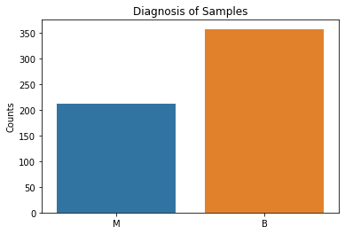
Our target variable has approximately 150 more benign samples than malignant samples. While it is expected that benign values would likely outnumber malignant values, this means that accuracy as a target metric for our machine learning algorithms will be deceptively high. We will focus on the F1, precision, and recall scores instead.

While these values are skewed which could affect the model, the outliers could also be possibly correlated with more malignant disease. I will not transform these skewed values to be as accurate as possible.

Using swarm plots, the numeric variables were compared with the target diagnosis of benign or malignant.

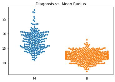
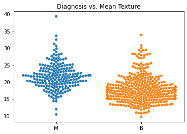
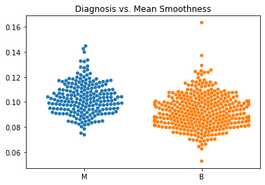
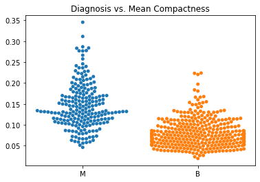
In general, the mean values for many of the predictor variables tended to be higher with malignant diagnoses versus benign diagnoses.

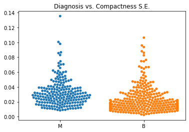
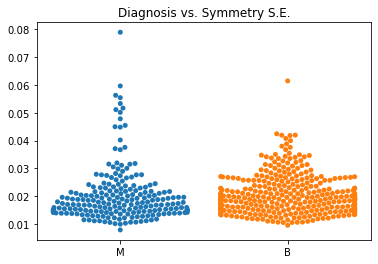
The standard error values for the predictors tended to be equivalent between the malignant and benign diagnoses.

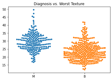
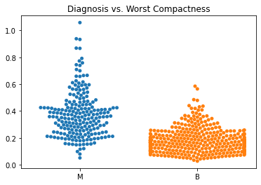
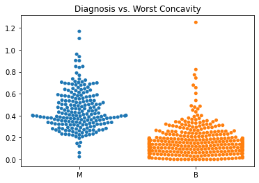
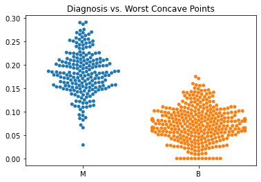
The malignant tumors seemed to have higher worst texture, compactness, concavity, and concave points.

Machine Learning Fitting and Prediction

In general, the goal of these machine learning algorithms would be to eliminate false negatives as much as possible. For example, we would not want our models to predict a benign diagnosis when a cancer was present. While false positives (predicting cancer when it is benign) would be quite distressing, it would not be as potentially devastating as a missed cancer diagnosis. The algorithms will be judged on this ability as well as Precision, Recall, and F1 scores.

Logistic Regression

#Running Logistic Regression Method to Predict Malignant or Benign

#Importing Packages
from sklearn.model_selection import train_test_split
from sklearn.linear_model import LogisticRegression
from sklearn.preprocessing import StandardScaler
from sklearn.metrics import classification_report, confusion_matrix

#Creating Features and Target Objects
features = df.loc[:, df.columns != 'diagnosis']
target = df['diagnosis']

#Creating Standardizer
standardizer = StandardScaler()

#Creating Logistic Regression Object
logit = LogisticRegression()

#Standardizing Features
features_standardized = standardizer.fit_transform(features)

#Train Test 80/20 Split
features_train, features_test, target_train, target_test = train_test_split(features_standardized, target, test_size = 0.2, random_state =1)

#Fitting Data to Logistic Regression Classifier
logreg = logit.fit(features_train, target_train)

#Generating Confusion Matrix/Classification Report
target_pred = logit.predict(features_test)
test0 = np.array(target_test)
predictions0 = np.array(target_pred)
print("Confusion Matrix:\n", confusion_matrix(test0, predictions0),'\n')
print("Classification Report:\n", classification_report(test0, predictions0))

Confusion Matrix:
 [[71  1]
 [ 2 40]]

Classification Report:
               precision    recall  f1-score   support

           B       0.97      0.99      0.98        72
           M       0.98      0.95      0.96        42

    accuracy                           0.97       114
   macro avg       0.97      0.97      0.97       114
weighted avg       0.97      0.97      0.97       114

This model performed quite well. There were 2 misclassifications of benign lesions that were actually malignant. F1 score for benign lesions was 0.98 and malignant lesions was 0.96 which are quite high. Next we will check the feature importance of the different factors in the model based on their coefficients.

#Checking Feature Importance Based on Coefficients

#Importing Packages
from yellowbrick.model_selection import FeatureImportances

#Getting Labels and Checking Feature Importances For Logistic Regression Model
labels = list(map(lambda x: x.title(), features))
viz = FeatureImportances(logreg, labels=labels)
viz.fit(features_train, features_test)
viz.show()

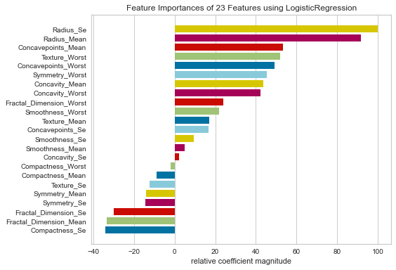
Looking at the relative feature importance using the logistic regression model, radius_se, radius_mean, concavepoints_mean, texture/concavepoints/symmetry worst and concavity_mean/worst all had fairly high relative importances based on their coefficients.

It is not surprising that the radius mean and standard error values were highly important in the model since cell size can be proportional to malignant cells. It is also interesting that there were a lot of variables with worst values that were highly important. This could suggest that the values that are the most abnormal could be associated with predicting malignant or benign lesions.

K Nearest Neighbors

First the data was fit on the KNN model and then the hyperparameters were optimized.

#Running KNN To Predict Malignant or Benign

#Using Same Features and Target as Previous Example though Will Need to Get Dummy Variables for Target
target = pd.get_dummies(df['diagnosis'])

#Importing Packages
from sklearn.neighbors import KNeighborsClassifier
from sklearn.model_selection import GridSearchCV, RandomizedSearchCV

#Creating Standardizer
standardizer = StandardScaler()

#Standardizing Features
features_standardized = standardizer.fit_transform(features)

#Train/Teset 80/20 Split
features_train, features_test, target_train, target_test = train_test_split(features_standardized, target, test_size = 0.2, random_state = 1)

#Creating KNN Object With K of 3 Before Hyperparameter Tuning
knn = KNeighborsClassifier(n_neighbors = 3, n_jobs = -1)

#Fitting Classifier on Training Data
knn.fit(features_train, target_train)

#Creating Confusion Matrix/Classification Report
target_pred = knn.predict(features_test)
test = np.array(target_test).argmax(axis=1)
predictions = np.array(target_pred).argmax(axis=1)
print("Confusion Matrix:\n", confusion_matrix(test, predictions),'\n')
print("Classification Report:\n", classification_report(test, predictions))

Confusion Matrix:
 [[69  3]
 [ 7 35]]

Classification Report:
               precision    recall  f1-score   support

           0       0.91      0.96      0.93        72
           1       0.92      0.83      0.88        42

    accuracy                           0.91       114
   macro avg       0.91      0.90      0.90       114
weighted avg       0.91      0.91      0.91       114

Using the following hyperparameters, the KNN model was re-run.

Best Leaf Size: 1
Best p: 1
Best n_neighbors: 7
Best Metric: minkowski
Best Weights: uniform


Confusion Matrix:
 [[70  2]
 [ 7 35]]

Classification Report:
               precision    recall  f1-score   support

           0       0.91      0.97      0.94        72
           1       0.95      0.83      0.89        42

    accuracy                           0.92       114
   macro avg       0.93      0.90      0.91       114
weighted avg       0.92      0.92      0.92       114

Feature importance was not done on the KNN model since it is not directly applicable to this algorithm. However, this model performed worse than the logistic regression model with F1-scores of 0.94 for benign lesions and 0.89 for malignant lesions. There were also 7 false negatives, which is much higher than the Logistic Regression model.

Random Forest Classifier

#Running Random Forest Algorithm on Data

#Importing Packages
from sklearn.ensemble import RandomForestClassifier

#Resetting Features and Targets
features = df.loc[:, df.columns != 'diagnosis']
target = df['diagnosis']

#Creating Standardizer
standardizer = StandardScaler()

#Standardizing Features
features_standardized = standardizer.fit_transform(features)

#Train/Teset 80/20 Split
features_train, features_test, target_train, target_test = train_test_split(features_standardized, target, test_size = 0.2, random_state = 1)

#Creating Random Forest Object
rf = RandomForestClassifier(n_estimators= 100, random_state = 1)

#Fitting Classifier on Training Data
rf.fit(features_train, target_train)

#Creating Confusion Matrix/Classification Report
target_pred = rf.predict(features_test)
test = np.array(target_test)
predictions = np.array(target_pred)
print("Confusion Matrix:\n", confusion_matrix(test, predictions),'\n')
print("Classification Report:\n", classification_report(test, predictions))

Confusion Matrix:
 [[72  0]
 [ 5 37]]

Classification Report:
               precision    recall  f1-score   support

           B       0.94      1.00      0.97        72
           M       1.00      0.88      0.94        42

    accuracy                           0.96       114
   macro avg       0.97      0.94      0.95       114
weighted avg       0.96      0.96      0.96       114

The random forest model performed slightly better than the KNN model with an F1 score of 0.97 for benign lesions and an F1 score of 0.94 for malignant lesions. Of more concern is that 5 benign lesions were classified as benign when they were actually malignant.

Next, for comparison between this and the logistic regression model, we’ll rank feature importance in this model as well.

#Ranking Feature Importance Based on the Random Forest Algorithm

labels1 = list(map(lambda x: x.title(), features))
viz = FeatureImportances(rf, labels=labels)
viz.fit(features_train, features_test)
viz.show()

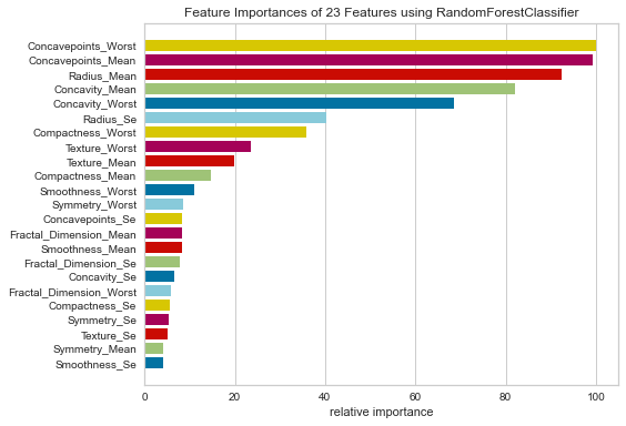
The results of this were quite interesting as well. Concavepoints_worst, concavepoints_mean, radius_mean, concavity_mean, and concavity_worst were all ranked highly with relative importance. These are very similar to the logistic regression model.

This would seem to suggest that radius_mean and concavepoints_worst/mean all seem to be important whichever model you are using and perhaps could be a focus of future projects.

Overall, the Logistic Regression model seems to be the best option of the three models tested. Due to the imbalanced target class, accuracy alone is not a good measure of performance since in an unbalanced class, the algorithm by chance could be more likely to guess a certain outcome because it knows that that is the most likely answer.

The F1 scores for the Logistic Regression model were the highest of the 3 models tested. This model also minimized the number of false negatives or missed cancer diagnoses.

Limitations of this dataset include older data as well as limited data points. Further projects would require thousands, perhaps millions of more current data points. Healthcare demographics as well as cancer diagnosis and treatment standards of care change rapidly so current data is paramount.

This project demonstrates that machine learning could be potentially useful as an adjunct to standard patient care. The goal should be to use machine learning models as an adjunct to flag potentially high-risk findings that should be further investigated before disregarding. This could be something as simple as the model indicating that there are several highly suspicious features of malignancy and have a physician review for final diagnosis to either concur or dispute that result.

For full code of the project, please refer to my GitHub repository under Applied Data Science.