Heart Failure Survival Prediction

Heart Failure Survival Prediction

Brandon May

Cardiovascular disease is still an important cause of morbidity and mortality worldwide. Heart failure, which is an inability for the heart to pump blood efficiency can easily be fatal and diagnosis can be challenging. While traditional machine learning has not been extensively used in clinical medicine outside of academic research environments, there are many different applications of this.

Heart failure can be particularly devastating and caused by a wide variety of different clinical entities and many times, the cause is unknown. Certain therapies have been shown to improve outcomes in heart failure but is there a way to better detect mortality from heart failure to perhaps increase monitoring and intensify management of heart failure patients? This is the goal of this machine learning project.

Dataset Description:

This project focuses on a dataset that was used in the medical journal of BMC Medical Informatics and Decision Making. The citation of the dataset and the research article is pubilicly available by PLOS.

The dataset can be found at the following URL:

https://plos.figshare.com/articles/Survival_analysis_of_heart_failure_patients_A_case_study/5227684/1

The target variable in the dataset is classified as Event with 1 signifying death in the study. All subjects in this study were diagnosed with heart failure. There were otherwise 12 other features to use in the prediction of death including age, gender, smoking status, diabetes, anemia, ejection fraction, sodium level, creatinine, CPK, and platelets.

Reference Cited:

Chicco, D., & Jurman, G. (2020). Machine learning can predict survival of patients with heart failure from serum creatinine and ejection fraction alone. BMC Medical Informatics and Decision Making, 20(1). doi:10.1186/s12911-020-1023-5

Data Cleaning, Exploration, and Analysis

#Loading Basic Packages
import pandas as pd
import numpy as np
import matplotlib.pyplot as plt

#Silencing Warnings
import warnings
warnings.filterwarnings('ignore')

#Importing Dataset and Viewing
df = pd.read_csv("heart_failure_prediction.csv")
df

	TIME	Event	Gender	Smoking	Diabetes	BP	Anaemia	Age	Ejection.Fraction	Sodium	Creatinine	Pletelets	CPK
0	97	0	0	0	0	0	1	43.0	50	135	1.30	237000.00	358
1	180	0	1	1	1	0	1	73.0	30	142	1.18	160000.00	231
2	31	1	1	1	0	1	0	70.0	20	134	1.83	263358.03	582
3	87	0	1	0	0	0	1	65.0	25	141	1.10	298000.00	305
4	113	0	1	0	0	0	0	64.0	60	137	1.00	242000.00	1610
...	...	...	...	...	...	...	...	...	...	...	...	...	...
294	250	0	0	0	1	0	0	45.0	55	132	1.00	543000.00	582
295	244	0	0	0	1	0	0	51.0	40	134	0.90	221000.00	582
296	14	1	1	0	0	0	0	45.0	14	127	0.80	166000.00	582
297	80	0	1	0	1	0	0	60.0	45	133	1.00	297000.00	897
298	16	0	0	0	0	1	1	65.0	25	137	1.30	276000.00	52

299 rows × 13 columns

df.isnull().values.any()

False

There are no missing values in the dataset.

#Renaming Columns for Simplicity

df = df.rename(columns={"TIME": "Time", "Anaemia": "Anemia", "Ejection.Fraction": "EF", "Pletelets": "Platelets"})
df

	Time	Event	Gender	Smoking	Diabetes	BP	Anemia	Age	EF	Sodium	Creatinine	Platelets	CPK
0	97	0	0	0	0	0	1	43.0	50	135	1.30	237000.00	358
1	180	0	1	1	1	0	1	73.0	30	142	1.18	160000.00	231
2	31	1	1	1	0	1	0	70.0	20	134	1.83	263358.03	582
3	87	0	1	0	0	0	1	65.0	25	141	1.10	298000.00	305
4	113	0	1	0	0	0	0	64.0	60	137	1.00	242000.00	1610
...	...	...	...	...	...	...	...	...	...	...	...	...	...
294	250	0	0	0	1	0	0	45.0	55	132	1.00	543000.00	582
295	244	0	0	0	1	0	0	51.0	40	134	0.90	221000.00	582
296	14	1	1	0	0	0	0	45.0	14	127	0.80	166000.00	582
297	80	0	1	0	1	0	0	60.0	45	133	1.00	297000.00	897
298	16	0	0	0	0	1	1	65.0	25	137	1.30	276000.00	52

299 rows × 13 columns

Description of the Variables

TIME: Integer, signifying length of follow-up in days.

Event: Categorical (0: Died, 1: Alive)

Gender: Categorical (0: Female, 1: Male)

Smoking: Categorical (0: Non-Smoker, 1: Smoker)

Diabetes: Categorical (0: No Diabetes, 1: Diabetes)

BP: Categorical (0: No Hypertension, 1: Has Hypertension)

Anaemia: Categorical (0: No Anemia, 1: Anemia)

Age: Float (in years)

Ejection.Fraction: Integer (percentage)

Sodium: Integer (mg/dL)

Creatinine: Float (mg/dL)

Platelets: Float (mg/dL)

CPK: Integer

#Checking Data Types and Encoding As Appropriate
df.dtypes

Time            int64
Event           int64
Gender          int64
Smoking         int64
Diabetes        int64
BP              int64
Anemia          int64
Age           float64
EF              int64
Sodium          int64
Creatinine    float64
Platelets     float64
CPK             int64
dtype: object

#Recoding Our Categorical Variables

df['Event'] = df['Event'].astype('category')
df['Gender'] = df['Gender'].astype('category')
df['Smoking'] = df['Smoking'].astype('category')
df['Diabetes'] = df['Diabetes'].astype('category')
df['BP'] = df['BP'].astype('category')
df['Anemia'] = df['Anemia'].astype('category')

#Making Sure Coded Correctly
df.dtypes

Time             int64
Event         category
Gender        category
Smoking       category
Diabetes      category
BP            category
Anemia        category
Age            float64
EF               int64
Sodium           int64
Creatinine     float64
Platelets      float64
CPK              int64
dtype: object

print('Description of Numerical Categories')
df.describe()

Description of Numerical Categories

	Time	Age	EF	Sodium	Creatinine	Platelets	CPK
count	299.000000	299.000000	299.000000	299.000000	299.00000	299.000000	299.000000
mean	130.260870	60.833893	38.083612	136.625418	1.39388	263358.029264	581.839465
std	77.614208	11.894809	11.834841	4.412477	1.03451	97804.236869	970.287881
min	4.000000	40.000000	14.000000	113.000000	0.50000	25100.000000	23.000000
25%	73.000000	51.000000	30.000000	134.000000	0.90000	212500.000000	116.500000
50%	115.000000	60.000000	38.000000	137.000000	1.10000	262000.000000	250.000000
75%	203.000000	70.000000	45.000000	140.000000	1.40000	303500.000000	582.000000
max	285.000000	95.000000	80.000000	148.000000	9.40000	850000.000000	7861.000000

The numerical variables have some interesting descriptive statistics. The lowest age was 40 and the oldest person was 95. The lowest ejection fraction was 14% and the maximum was 80%. There was a significantly low sodium value of 113 and a high level of 148. For reference, normal sodium levels are between 135-145. The highest creatinine was 9.4 which is exceedingly high approaching renal failure range. Likewise, the lowest platelets of 25K and the highest were 850000. CPK, a muscle enzyme, had minimums of 23K with maximum of 7800K.

Looking at the means, the mean follow-up time was 130 days, age 60, EF of 38%, sodium of 136, creatinine of 1.39 (slightly elevated), 263K platelets (which is normal), and CPK of 481.

print('Description of Categorical Variables')
df.describe(include=['category'])

Description of Categorical Variables

	Event	Gender	Smoking	Diabetes	BP	Anemia
count	299	299	299	299	299	299
unique	2	2	2	2	2	2
top	0	1	0	0	0	0
freq	203	194	203	174	194	170

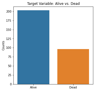
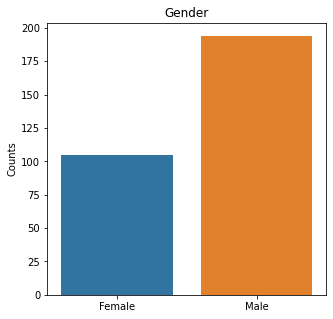
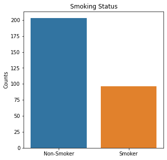
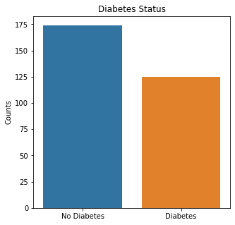
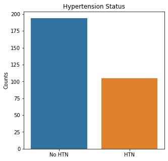
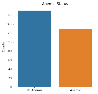
Based on the categorical variables, more patients were alive, male, non-smokers, non-diabetic, non-anemic, and with normal blood pressure.

#Searching for High Correlations
corr_matrix = df.corr()
corr_matrix

	Time	Age	EF	Sodium	Creatinine	Platelets	CPK
Time	1.000000	-0.224068	0.041729	0.087640	-0.149315	0.010514	-0.009346
Age	-0.224068	1.000000	0.060098	-0.045966	0.159187	-0.052354	-0.081584
EF	0.041729	0.060098	1.000000	0.175902	-0.011302	0.072177	-0.044080
Sodium	0.087640	-0.045966	0.175902	1.000000	-0.189095	0.062125	0.059550
Creatinine	-0.149315	0.159187	-0.011302	-0.189095	1.000000	-0.041198	-0.016408
Platelets	0.010514	-0.052354	0.072177	0.062125	-0.041198	1.000000	0.024463
CPK	-0.009346	-0.081584	-0.044080	0.059550	-0.016408	0.024463	1.000000

#Displaying Heat Map
plt.rcParams['figure.figsize'] = (5,5)

#Importing Seaborn
import seaborn as sns

sns.heatmap(corr_matrix)
plt.show()

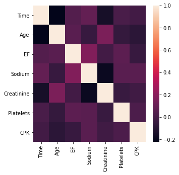
There do not appear to be any highly correlated variables.

#Creating Dataset with Categorical Only and Numerical Only

df_cat = df.drop(columns=['Time', 'Age', 'EF', 'Sodium', 'Creatinine', 'Platelets', 'CPK'])
df_num = df.drop(columns=['Event', 'Gender', 'Smoking', 'Diabetes', 'BP', 'Anemia'])

#Visualizing Numerical Data

#Setting Figure Size
plt.figure(figsize=[100,100])

f,a = plt.subplots(4,2, figsize=(60,30))

a = a.ravel()
for idx, ax in enumerate(a):
    ax.hist(df_num.iloc[:,idx], bins = 150)
    ax.set_title(df_num.columns[idx], size = 40)
    ax.set_ylabel('Counts', size = 20)
plt.show()

---------------------------------------------------------------------------

IndexError                                Traceback (most recent call last)

<ipython-input-12-384d7f5bdef4> in <module>
      8 a = a.ravel()
      9 for idx, ax in enumerate(a):
---> 10     ax.hist(df_num.iloc[:,idx], bins = 150)
     11     ax.set_title(df_num.columns[idx], size = 40)
     12     ax.set_ylabel('Counts', size = 20)


~\Anaconda\lib\site-packages\pandas\core\indexing.py in __getitem__(self, key)
   1760                 except (KeyError, IndexError, AttributeError):
   1761                     pass
-> 1762             return self._getitem_tuple(key)
   1763         else:
   1764             # we by definition only have the 0th axis


~\Anaconda\lib\site-packages\pandas\core\indexing.py in _getitem_tuple(self, tup)
   2065     def _getitem_tuple(self, tup: Tuple):
   2066 
-> 2067         self._has_valid_tuple(tup)
   2068         try:
   2069             return self._getitem_lowerdim(tup)


~\Anaconda\lib\site-packages\pandas\core\indexing.py in _has_valid_tuple(self, key)
    701                 raise IndexingError("Too many indexers")
    702             try:
--> 703                 self._validate_key(k, i)
    704             except ValueError:
    705                 raise ValueError(


~\Anaconda\lib\site-packages\pandas\core\indexing.py in _validate_key(self, key, axis)
   1992             return
   1993         elif is_integer(key):
-> 1994             self._validate_integer(key, axis)
   1995         elif isinstance(key, tuple):
   1996             # a tuple should already have been caught by this point


~\Anaconda\lib\site-packages\pandas\core\indexing.py in _validate_integer(self, key, axis)
   2061         len_axis = len(self.obj._get_axis(axis))
   2062         if key >= len_axis or key < -len_axis:
-> 2063             raise IndexError("single positional indexer is out-of-bounds")
   2064 
   2065     def _getitem_tuple(self, tup: Tuple):


IndexError: single positional indexer is out-of-bounds



<Figure size 7200x7200 with 0 Axes>

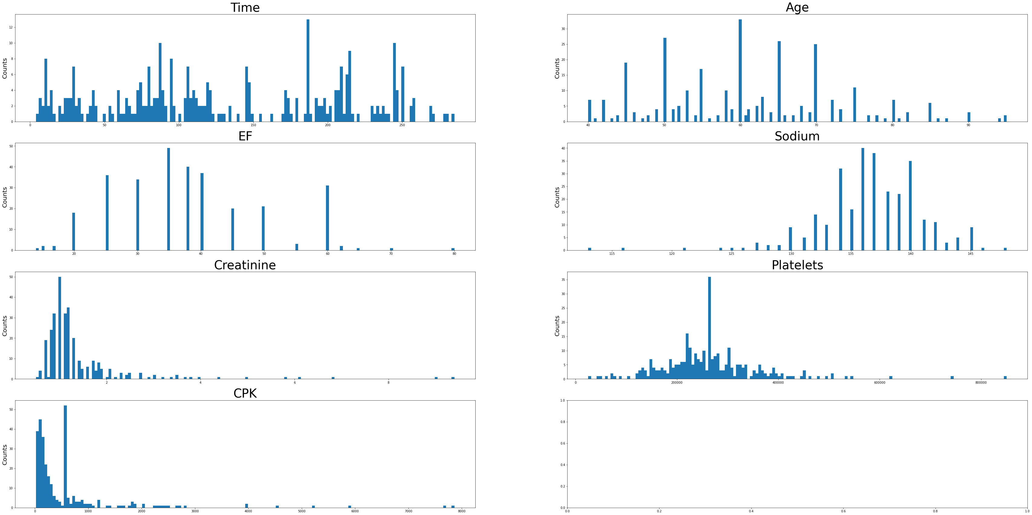
Sodium levels have positive skew, while creatinine, platelets, EF, and CPK levels appear negatively skewed. The Time variable has a multimodal distribution. Age looks to be approximately normally distributed with a slight positive skew.

#Visualizing Categorical Data

sns.countplot(x = 'Event', data = df_cat)
plt.title('Target Variable: Alive vs. Dead')
plt.xticks([0,1], ['Alive', 'Dead'])
plt.xlabel(xlabel = None)
plt.ylabel('Counts')
plt.show()

sns.countplot(x = 'Gender', data = df_cat)
plt.title('Gender')
plt.xticks([0,1], ['Female', 'Male'])
plt.xlabel(xlabel=None)
plt.ylabel('Counts')
plt.show()

sns.countplot(x = 'Smoking', data = df_cat)
plt.title('Smoking Status')
plt.xticks([0,1], ['Non-Smoker', 'Smoker'])
plt.xlabel(xlabel=None)
plt.ylabel('Counts')
plt.show()

sns.countplot(x = 'Diabetes', data = df_cat)
plt.title('Diabetes Status')
plt.xticks([0,1], ['No Diabetes', 'Diabetes'])
plt.xlabel(xlabel=None)
plt.ylabel('Counts')
plt.show()

sns.countplot(x = 'BP', data = df_cat)
plt.title('Hypertension Status')
plt.xticks([0,1], ['No HTN', 'HTN'])
plt.xlabel(xlabel=None)
plt.ylabel('Counts')
plt.show()

sns.countplot(x = 'Anemia', data = df_cat)
plt.title('Anemia Status')
plt.xticks([0,1], ['No Anemia', 'Anemic'])
plt.xlabel(xlabel=None)
plt.ylabel('Counts')
plt.show()

#Visualizing Boxplots to Assess for Outliers

plt.boxplot(df['Time'])
plt.title('Boxplot of Time Follow-Up Variable')
plt.ylabel('Time (Days)')
plt.show()

plt.boxplot(df['Age'])
plt.title('Boxplot of Age Variable')
plt.ylabel('Age (years)')
plt.show()

plt.boxplot(df['EF'])
plt.title('Boxplot of EF')
plt.ylabel('EF (%)')
plt.show()

plt.boxplot(df['Sodium'])
plt.title('Boxplot of Sodium Level')
plt.ylabel('Sodium (mg/dL)')
plt.show()

plt.boxplot(df['Creatinine'])
plt.title('Boxplot of Creatinine')
plt.ylabel('Creatinine (mg/dL)')
plt.show()

plt.boxplot(df['Platelets'])
plt.title('Boxplot of Platelets')
plt.ylabel('Platelets (mg/dL)')
plt.show()

plt.boxplot(df['CPK'])
plt.title('Boxplot of CPK Level')
plt.ylabel('CPK (mg/dL)')
plt.show()

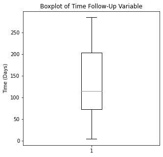
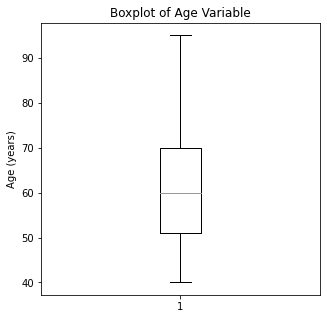
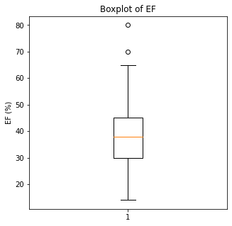
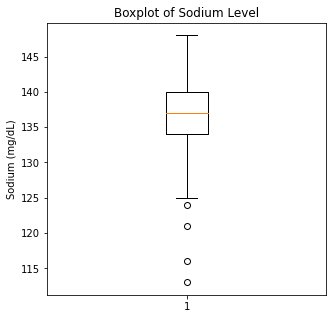
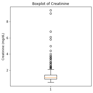
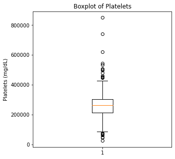
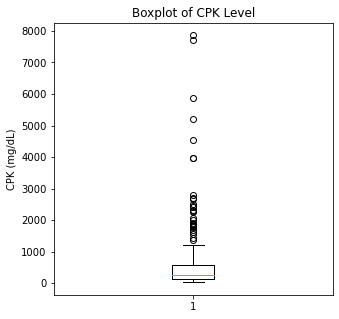
There are some significant outliers in these variables, specifically regarding creatinine levels, CPK, platelet levels, and to some extent sodium levels. We will keep these outliers in the dataset as these significant outliers could be predictive of worse prognosis and deleting them would affect our algorithms.

#Visualizing Swarm Plots to Compare The Target Variable to Our Explanatory Variables

categories = df.Event

sns.swarmplot(categories, df.Time)
plt.title('Survival vs. Follow-Up Time')
plt.xlabel(xlabel = None)
plt.ylabel('Follow-Up (Days)')
plt.xticks([0,1], ['Alive', 'Dead'])
plt.show()

sns.swarmplot(categories, df.Age)
plt.title('Survival vs. Age')
plt.xlabel(xlabel = None)
plt.ylabel('Age (years)')
plt.xticks([0,1], ['Alive', 'Dead'])
plt.show()

sns.swarmplot(categories, df.EF)
plt.title('Survival vs. Ejection Fraction')
plt.xlabel(xlabel = None)
plt.ylabel('Ejection Fraction (%)')
plt.xticks([0,1], ['Alive', 'Dead'])
plt.show()

sns.swarmplot(categories, df.Sodium)
plt.title('Survival vs. Sodium Level')
plt.xlabel(xlabel = None)
plt.ylabel('Sodium Level (mg/dL)')
plt.xticks([0,1], ['Alive', 'Dead'])
plt.show()

sns.swarmplot(categories, df.Creatinine)
plt.title('Survival vs. Creatinine Level')
plt.xlabel(xlabel = None)
plt.ylabel('Creatinine (mg/dL)')
plt.xticks([0,1], ['Alive', 'Dead'])
plt.show()

sns.swarmplot(categories, df.Platelets)
plt.title('Survival vs. Platelets Level')
plt.xlabel(xlabel = None)
plt.ylabel('Platelets (mg/dL)')
plt.xticks([0,1], ['Alive', 'Dead'])
plt.show()

sns.swarmplot(categories, df.CPK)
plt.title('Survival vs. CPK Level')
plt.xlabel(xlabel = None)
plt.ylabel('CPK (mg/dL)')
plt.xticks([0,1], ['Alive', 'Dead'])
plt.show()

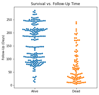
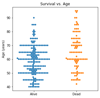
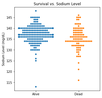
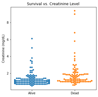
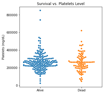
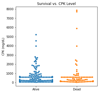
There are several interesting findings when plotting survival vs our different numerical variables. Unsurprisingly, those who had longer follow-up in days were more likely to be alive. There was a trend that the older individuals were more likely to not have survived. It is subtle, but there appears to be an association between lower EF and survival and this is logical however, looking at the distributions, there was not a significant difference between the two. Likewise, there did not seem to be a significant difference between sodium level and survival. The higher the level of creatinine above 2, the more likely they were to be dead. These creatinine levels are exceedingly high and the higher the creatinine, the higher the likelihood of kidney failure which explains this trend. There did not seem to be a significant difference between survival and the platelet/CPK levels.

Machine Learning Algorithms

In general, when fitting the data using various models, the false negatives or predicting survival when the patient could be at risk of death should be minimized if at all possible. The risk of predicting someone who is at higher risk of death who truly is not at risk would not be as catastrophic as a false negative. The algorithms were evaluated using precision, recall, F1 scores, and ROC curves.

Logistic Regression

#Importing Packages
from sklearn.model_selection import train_test_split
from sklearn.linear_model import LogisticRegression
from sklearn.preprocessing import StandardScaler
from sklearn.metrics import classification

from yellowbrick.classifier import ConfusionMatrix, ClassificationReport, ROCAUC

#Creating Features and Target Objects
features = df.loc[:, df.columns != 'Event']
target = df['Event']

#Getting Dummies for Our Categoricals
features = pd.get_dummies(features)

#Creating Standardizer and Logit Objects
standardizer = StandardScaler()
logit = LogisticRegression()

#Standardizing Features
features_standardized = standardizer.fit_transform(features)

#Train/Test Split
features_train, features_test, target_train, target_test = train_test_split(features_standardized, target, test_size = 0.2)

#Fitting Data to Logistic Regression Classifier
logreg = logit.fit(features_train, target_train)

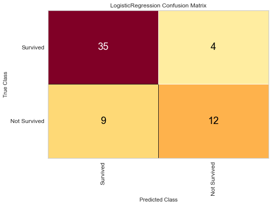
#Confusion Matrix Visualizer
classes = ['Survived', 'Not Survived']
cm = ConfusionMatrix(logit, classes = classes, percent = False)

#Fitting Passed Model
cm.fit(features_train, target_train)
cm.score(features_test, target_test)

#Changing Fontsize in Figure
for label in cm.ax.texts:
    label.set_size(20)
    
cm.poof()

#Configuring Graph Parameters
plt.rcParams['figure.figsize'] = (15,7)
plt.rcParams['font.size'] = 20

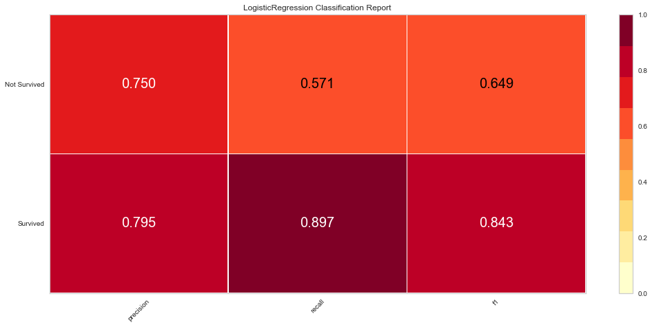
visualizer = ClassificationReport(logit, classes = classes)
visualizer.fit(features_train, target_train)
visualizer.score(features_test, target_test)
g = visualizer.poof()

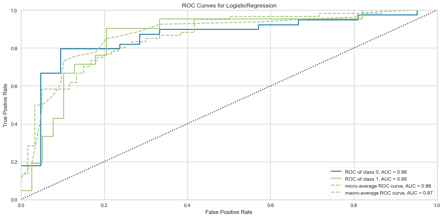
#ROC/AUC Curve

roc = ROCAUC(logit)
roc.fit(features_train, target_train)
roc.score(features_test, target_test)
g = roc.poof()

#Checking Variable Feature Importance

from yellowbrick.model_selection import FeatureImportances

#Getting Labels and Checking Feature Importance for Log Reg Model
labels = list(map(lambda x: x.title(), features))
viz = FeatureImportances(logreg, labels = labels)
viz.fit(features_train, features_test)
viz.show()

<matplotlib.axes._subplots.AxesSubplot at 0x145ab1b0e80>

The logistic regression model performed reasonably well with an F1 score of 0.615 of predicting death and 0.815 of predicting death. There were 8 false negatives in this model. The ROC was 0.81 for both class predictions. After checking feature importance based on the logistic regression model, age, creatinine, CPK levels, and female gender were some of the most important features based on relative coefficients.

KNN

#Importing Packages
from sklearn.neighbors import KNeighborsClassifier
from sklearn.model_selection import GridSearchCV, RandomizedSearchCV
from sklearn.metrics import classification_report, confusion_matrix

#Getting Dummies for Target Variable
target = pd.get_dummies(df['Event'])

#Train/Test 80/20 Split
features_train, features_test, target_train, target_test = train_test_split(features_standardized, target, test_size = 0.2, random_state = 1)

#Starting with KNN of 3
knn = KNeighborsClassifier(n_neighbors = 3, n_jobs = -1)
knn.fit(features_train, target_train)

#Visualizing Metrics
target_pred = knn.predict(features_test)
test = np.array(target_test).argmax(axis=1)
predictions = np.array(target_pred).argmax(axis=1)
print('Confusion Matrix:\n', confusion_matrix(test, predictions), '\n')
print('Classification Report:\n', classification_report(test, predictions), '\n')

Confusion Matrix:
 [[34  7]
 [11  8]] 

Classification Report:
               precision    recall  f1-score   support

           0       0.76      0.83      0.79        41
           1       0.53      0.42      0.47        19

    accuracy                           0.70        60
   macro avg       0.64      0.63      0.63        60
weighted avg       0.69      0.70      0.69        60

#Hyperparameter Tuning for KNN Using GridSearch CV

param_dist = {"leaf_size": list(range(1,50)),
             "n_neighbors": list(range(1,30)),
             "p": [1,2]}

#Using GridSearch Object
clf = GridSearchCV(knn, param_dist, cv=10, n_jobs = -1)
best_model = clf.fit(features_standardized, target)

print('Best Leaf Size:', best_model.best_estimator_.get_params()['leaf_size'])
print('Best p:', best_model.best_estimator_.get_params()['p'])
print('Best n_neighbors:', best_model.best_estimator_.get_params()['n_neighbors'])
print('Best Metric:', best_model.best_estimator_.get_params()['metric'])
print('Best Weights:', best_model.best_estimator_.get_params()['weights'])

Best Leaf Size: 1
Best p: 2
Best n_neighbors: 5
Best Metric: minkowski
Best Weights: uniform

#Running New Tuned Model and Evaluating Metrics
knn_best = KNeighborsClassifier(n_neighbors = 5, p = 1, leaf_size = 1, metric = "minkowski", weights= "uniform", n_jobs = -1)
knn_best.fit(features_train, target_train)
target_pred = knn_best.predict(features_test)
test = np.array(target_test).argmax(axis=1)
predictions = np.array(target_pred).argmax(axis=1)
print("Confusion Matrix:\n", confusion_matrix(test, predictions),'\n')
print("Classification Report:\n", classification_report(test, predictions))

Confusion Matrix:
 [[36  5]
 [13  6]] 

Classification Report:
               precision    recall  f1-score   support

           0       0.73      0.88      0.80        41
           1       0.55      0.32      0.40        19

    accuracy                           0.70        60
   macro avg       0.64      0.60      0.60        60
weighted avg       0.67      0.70      0.67        60

Using the tuned hyperparameters, interestingly, this model had better success at predicting death than survival. However, there were 13 false negatives which we would want to avoid. The F1 scores are not as high as the logistic regression model unfortunately.

Support Vector Machine Classifier

#Importing Packages
from sklearn.svm import SVC

#Resetting our Target Object to Not Have Dummy Variables
target = df['Event']

#Creating SVM Object
svc = SVC(kernel='linear')

#Train/Test 80/20 Split
features_train, features_test, target_train, target_test = train_test_split(features_standardized, target, test_size = 0.2, random_state = 1)

svc.fit(features_train, target_train)

cm_svc = ConfusionMatrix(svc, classes = classes, percent = False)
cm_svc.fit(features_train, target_train)
cm_svc.score(features_test, target_test)
cm_svc.poof()

svc_vis = ClassificationReport(svc, classes = classes)
svc_vis.fit(features_train, target_train)
svc_vis.score(features_test, target_test)
svc_vis.poof()

svc_roc = ROCAUC(svc, micro = False, macro = False, per_class = False)
svc_roc.fit(features_train, target_train)
svc_roc.score(features_test, target_test)
svc_roc.poof()

<matplotlib.axes._subplots.AxesSubplot at 0x145a9b8f970>

#Checking Feature Importance
labels = list(map(lambda x: x.title(), features))
viz = FeatureImportances(svc, labels = labels)
viz.fit(features_train, features_test)
viz.show()

<matplotlib.axes._subplots.AxesSubplot at 0x145a9c5d310>

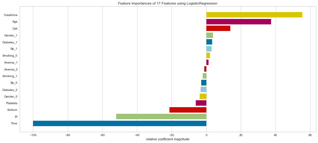
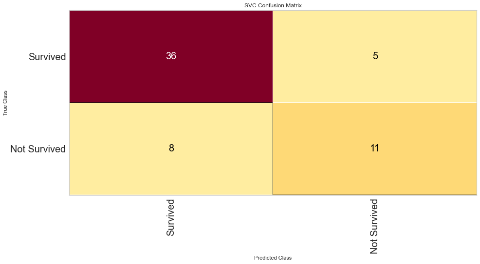
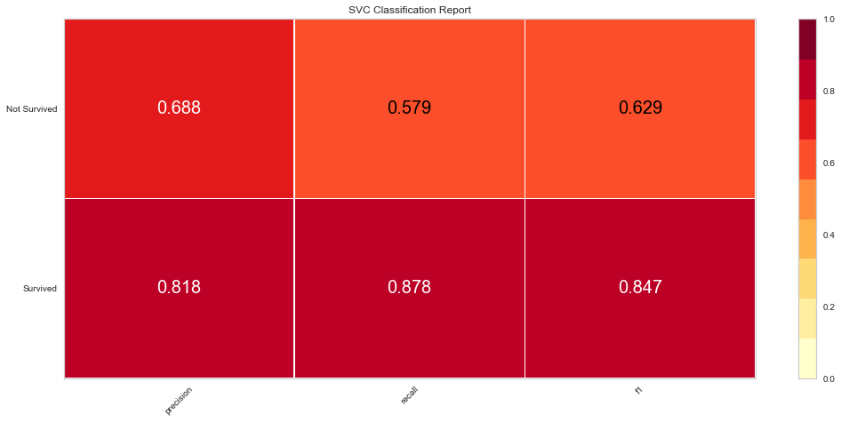
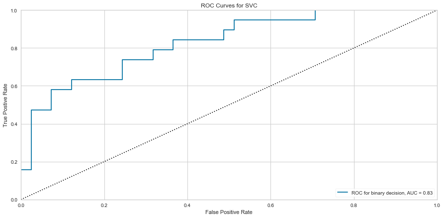
Support vector machine was run using the same parameters. This model had a low number of false negatives at 8 people incorrectly predicted. The F1 scores were higher than the logistic regression model at 0.847 for predicting survival and 0.629 for predicting death. The ROC was slightly better at 0.83. Overall, this appears to be marginally better. Checking feature importance, creatinine, age, cpk, and female gender were all highly important. The one difference is that the presence of anemia and current smoking also appeared to be relatively important in the model.

Random Forest

#Importing Packages
from sklearn.ensemble import RandomForestClassifier

#Resetting Features and Targets
features = df.loc[:, df.columns != 'Event']
target = df['Event']

#Train/Test 80/20 Split
features_train, features_test, target_train, target_test = train_test_split(features, target, test_size = 0.2)

#Creating Object
rfc = RandomForestClassifier(n_estimators = 100, random_state = 1)
rfc.fit(features_train, target_train)

#Visualizing Confusion Matrix, Class Report, and ROC Curve
rfc_cm = ConfusionMatrix(rfc, classes = classes, percent = False)
rfc_cm.fit(features_train, target_train)
rfc_cm.score(features_test, target_test)
rfc_cm.poof()

rfc_class = ClassificationReport(rfc, classes = classes)
rfc_class.fit(features_train, target_train)
rfc_class.score(features_test, target_test)
rfc_class.poof()

rfc_roc = ROCAUC(rfc)
rfc_roc.fit(features_train, target_train)
rfc_roc.score(features_test, target_test)
rfc_roc.poof()

<matplotlib.axes._subplots.AxesSubplot at 0x145adafefa0>

#Checking Feature Importance
labels = list(map(lambda x: x.title(), features))
viz = FeatureImportances(rfc, labels = labels)
viz.fit(features_train, features_test)
viz.show()

<matplotlib.axes._subplots.AxesSubplot at 0x145ada11250>

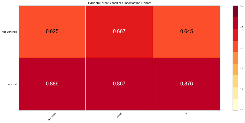
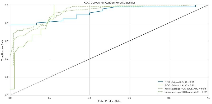
This model performed quite well. It had only 4 false negatives and an F1 score of 0.70 for predicting death, and 0.884 for predicting survival. The ROC was 0.90 for both classes.

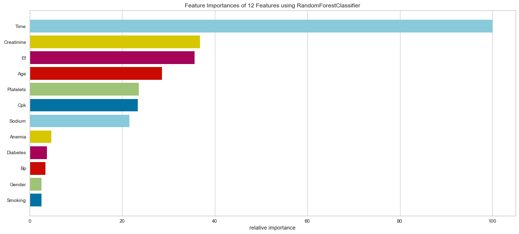
It is interesting that in this model, the ensemble method put a high weight on follow-up time. Creatinine, EF, CPK, Age, Platelets, and Sodium levels were all highly important. Gender was less important in this model. This result is interesting in that EF is directly tied to prognosis in heart failure patients and sodium level can be indicative of fluid balance. Abnormal sodium levels can indicate worsening heart failure symptoms, so this makes medical sense.

XG Boost

#Importing Packages
from xgboost import XGBClassifier

features = pd.get_dummies(features)
target = df['Event']

#Train/Test 80/20 Split
features_train, features_test, target_train, target_test = train_test_split(features, target, test_size = 0.2)

xgb = XGBClassifier(random_state = 1)
xgb.fit(features_train, target_train)

#Visualizing Confusion Matrix, Class Report, and ROC Curve
xgb_cm = ConfusionMatrix(xgb, classes = classes, percent = False)
xgb_cm.fit(features_train, target_train)
xgb_cm.score(features_test, target_test)
xgb_cm.poof()

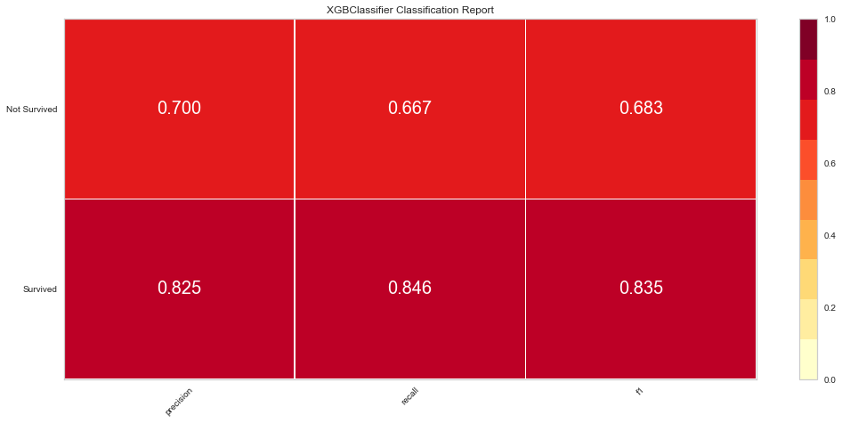
xgb_class = ClassificationReport(xgb, classes = classes)
xgb_class.fit(features_train, target_train)
xgb_class.score(features_test, target_test)
xgb_class.poof()

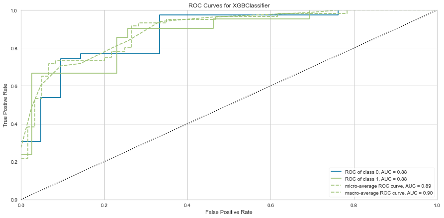
xgb_roc = ROCAUC(xgb)
xgb_roc.fit(features_train, target_train)
xgb_roc.score(features_test, target_test)
xgb_roc.poof()

<matplotlib.axes._subplots.AxesSubplot at 0x145baabf310>

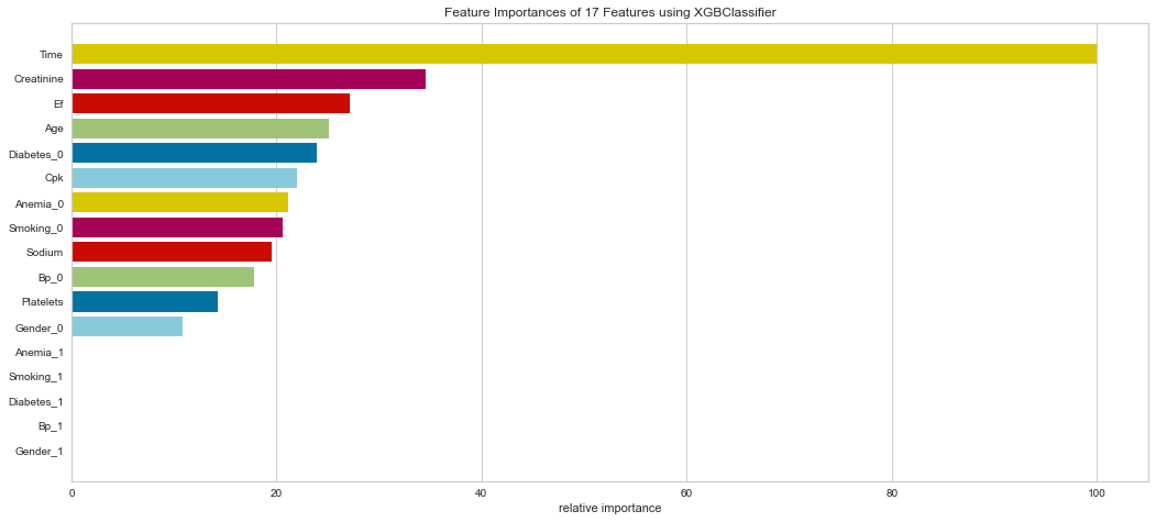
#Checking Feature Importance
labels = list(map(lambda x: x.title(), features))
viz = FeatureImportances(xgb, labels = labels)
viz.fit(features_train, features_test)
viz.show()

<matplotlib.axes._subplots.AxesSubplot at 0x145aad585e0>

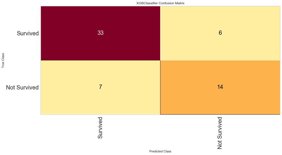
This model also performed quite well. There were only 4 false negatives. The F1 score for predicting death was 0.769 and predicting survival was 0.889. The ROC was 0.92. Feature importance showed a similar result to the Random Forest method showing that time of follow-up, creatinine, EF, female gender, age, and sodium level were all important among several others.

Conclusions

Heart failure is a very deadly disease. Even 20 years ago, this diagnosis would be a death sentence. There have been significant pharmacologic advancements in recent years which have improved survival. Those with heart failure can have hospital admissions for fluid overload, trouble breathing, and even other cardiac events. However, heart failure survival is still dependent upon the severity of the symptoms and other objective measurements as well as early diagnosis and treatment (Colucci, 2019). Therefore, it is timely that we may be able to utilize machine learning algorithms to help better predict death. Perhaps if we can predict a higher risk of death based on severity of various lab measurements and other risk factors, there could be an intensification of therapy and/or aggressive follow-up and monitoring to ensure adequate care and prolonged symptom-free survival.

It is not a significant surprise that the Random Forest and XG Boost models performed the best based on ROC and F1 scores. The Random Forest managed to edge out the XG Boost performance by a small margin. Since both of these are ensemble methods, they have multiple algorithms that are being evaluated and the prediction is then confirmed using a majority vote option. Which model to use is somewhat arbitrary given their largely similar results.

In this population of patients, there were significantly more people alive than dead at the end of the study period. This explains why many of the models predicted more to be alive than dead on a relative basis. The ensemble methods performed the best at this showing the power of these algorithm to be able to predict the harder class (death). This is the point of this project; we want to primarily identify those at high risk of mortality to either perform some sort of intervention or close monitoring. However, predicting survival can also be beneficial in that if a patient were to be predicted to survive by certain criteria, you could ensure certain factors about their health are optimized and be reassured.

Finally, it is fascinating that the machine learning algorithms all seemed to agree on certain variables that relatively more important to the prediction. The majority of them noted age, creatinine, CPK, and female gender to have more predictive power. The ensemble methods picked up on more of the traditional variables of sodium, ejection fraction, among others. Many of these variables are already medically validated as related to heart failure prognosis. The machine learning algorithms, at least based on this dataset, agreed with these factors. These factors do differ slightly based on the different algorithms used but many of the algorithms picked out similar important variables.

This dataset is smaller and has a small number of patients. This is partly due to the low numbers of heart failure overall. This is a limitation on the predictive power. Much larger datasets would be necessary among a large patient demographic to apply to the general population. This does continue to show that machine learning can aid healthcare workers and providers in clinical management.